
The familiar rule says save 25× your annual spending and withdraw 4% a year. We asked Retirement Lab a narrower question: for one household, holding purchasing power constant, how many years of local spending did the portfolio actually have to be to reach a 95% simulated success target over a 55-year retirement?
The answer was never 25×. Across all 31 tax-residence countries Retirement Lab supports, the required multiple ranged from 34.1× to 51.5× of local annual spending. Holding a portfolio of exactly 25× local spending instead, none of the 124 cases in the wider grid reached the 95% target; the best simulated result anywhere was 88.1%.
Two different things produce that gap, and it is worth separating them.
The floor: about 34×, before any tax at all
Four country cases in this set paid essentially no modelled tax in year one: the UAE, the US, the UK, and Malaysia. They landed at 34.1×, 34.3×, 35.3×, and 35.8× — an implied first-year withdrawal rate of roughly 2.8–2.9%, not 4%.
That floor has nothing to do with tax. It comes from three choices that differ from the rule's origin. William Bengen's 1994 study Determining Withdrawal Rates Using Historical Data (Journal of Financial Planning, October 1994) asked how large an inflation-adjusted withdrawal a portfolio of US stocks and intermediate Treasuries could sustain over 30 years of historical sequences, in pre-tax terms. This simulation runs 55 years (a couple retiring at 40 and planning to 95), targets 95% success rather than "never failed in the historical sample", draws returns from a fat-tailed distribution rather than resampled history, and charges each country's modelled tax along the way.
Lengthen the horizon, raise the bar, and fatten the left tail, and roughly 34× is what the same portfolio question produces — even when the tax bill is zero.
The spread: everything above the floor is tax
Once cost of living is normalised away, the difference between countries is almost entirely modelled tax treatment. The table below reports the $60,000 spending level. "Required portfolio" is in USD, but the multiple is against local spending — what $60,000 of US purchasing power costs in that country.
Each country links to the published scenario, so you can inspect the assumptions and fork it with your own numbers.
| Country | Required portfolio | Multiple of local spending | Implied first-year withdrawal | Simulated success at 25× | Year-one tax as % of spending |
|---|---|---|---|---|---|
| UAE | $1,430,000 | 34.1× | 2.93% | 88.1% | 0% |
| US | $2,060,000 | 34.3× | 2.91% | 88.1% | 0% |
| Chile | $1,060,000 | 34.5× | 2.90% | 87.7% | 1% |
| Canada | $1,890,000 | 34.8× | 2.88% | 87.2% | 7% |
| Thailand | $650,000 | 35.1× | 2.85% | 86.6% | 7% |
| Panama | $1,080,000 | 35.2× | 2.84% | 85.2% | 8% |
| Australia | $1,980,000 | 35.3× | 2.84% | 87.6% | 5% |
| Czechia | $1,370,000 | 35.3× | 2.83% | 85.4% | 8% |
| UK | $1,850,000 | 35.3× | 2.83% | 86.7% | 0% |
| South Africa | $900,000 | 35.7× | 2.80% | 86.7% | 9% |
| Malaysia | $680,000 | 35.8× | 2.79% | 87.3% | 0% |
| Costa Rica | $1,370,000 | 35.9× | 2.79% | 83.7% | 12% |
| Singapore | $1,680,000 | 35.9× | 2.79% | 87.7% | 2% |
| Switzerland | $2,730,000 | 36.2× | 2.76% | 85.3% | 17% |
| Vietnam | $570,000 | 36.2× | 2.76% | 87.3% | 3% |
| Malta | $1,380,000 | 36.4× | 2.75% | 85.8% | 10% |
| Mexico | $1,290,000 | 36.4× | 2.74% | 85.2% | 8% |
| Cyprus | $1,400,000 | 36.5× | 2.74% | 85.5% | 12% |
| Uruguay | $1,600,000 | 36.6× | 2.73% | 86.2% | 8% |
| Greece | $1,360,000 | 37.5× | 2.66% | 83.7% | 12% |
| Brazil | $1,070,000 | 38.1× | 2.63% | 83.7% | 12% |
| Belgium | $1,890,000 | 38.7× | 2.58% | 83.0% | 22% |
| Hungary | $1,210,000 | 39.0× | 2.57% | 81.3% | 23% |
| Spain | $1,500,000 | 39.2× | 2.55% | 81.2% | 24% |
| Japan | $1,550,000 | 39.4× | 2.54% | 81.6% | 17% |
| Austria | $1,920,000 | 41.0× | 2.44% | 78.7% | 25% |
| Portugal | $1,510,000 | 41.6× | 2.40% | 78.4% | 25% |
| France | $1,950,000 | 41.9× | 2.39% | 76.4% | 29% |
| Germany | $1,910,000 | 41.9× | 2.39% | 79.9% | 22% |
| Italy | $1,720,000 | 42.4× | 2.36% | 76.9% | 33% |
| Netherlands | $2,480,000 | 51.5× | 1.94% | 72.2% | 99% |
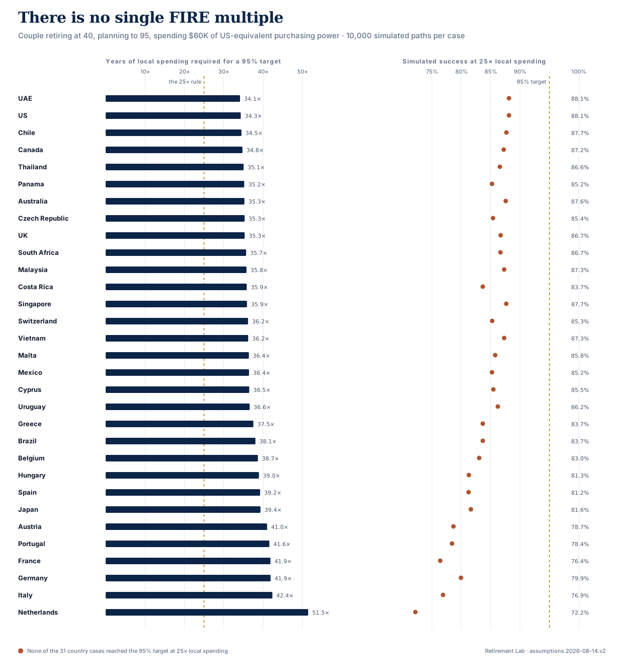
Both panels keep the same row order. The right panel is a separate set of runs at a portfolio of exactly 25× local spending; it does not reuse the probability from the threshold search.
Read the last two columns together. The year-one tax bill and the required multiple move broadly in lockstep — 0% at the top, around 12% in the middle, 33% for Italy, 99% for the Netherlands. That is what you would expect if tax, not cost of living and not luck, is what separates these countries once spending is held at equal purchasing power.
Why the cheap countries are not the cheap countries
Malaysia's required portfolio was $680,000 and Switzerland's was $2,730,000. That is a real and useful difference: it is what a $60,000 US lifestyle costs to fund in each place. But it is mostly a price-level fact, and it is the answer the 26-country ranking already gives.
Expressed as a multiple of local spending, the ordering nearly reverses. Malaysia needed 35.8× and Switzerland 36.2× — nearly identical, despite a fourfold difference in dollars, and both far from the 51.5× the Netherlands required.
The reason is that the cost-of-living adjustment does exactly one job: it shrinks the spending target. It does not make the country's tax code kinder. A household living on the Malaysian equivalent of $19,000 a year still faces Malaysia's tax treatment of its portfolio — which in this case happens to be nothing, because Malaysia does not tax foreign-source investment income for this household. That exemption is why Malaysia sits near the floor, and it depends on the portfolio being held outside Malaysia, which is the realistic case for someone who moved there.
The US result is worth checking by hand, because it anchors the top of the table. At the $2.06M threshold, a 2% dividend yield is about $41,200 of qualified dividends. A married couple filing jointly deducts the standard deduction from that, leaving taxable income inside the 0% long-term capital gains and qualified-dividend bracket. The simulation's modelled first-year federal tax is $0. Change the account mix — most of these dollars in a traditional 401(k) or IRA instead of a brokerage account — and that result changes substantially. See What this does not say.
The Netherlands is a different kind of tax
The Netherlands required 51.5× local spending and a 1.94% first-year withdrawal rate. It is not a near miss on the pack — it is 9.1× clear of Italy in second place.
The mechanism is that Box 3 taxes assets, not income. Retirement Lab models the 2026 regime: a deemed return of 6.00% on investments, a tax-free allowance of €59,357 per person, and a 36% rate (Belastingdienst). A charge on assets does not shrink when you spend less, which is why it dominates every other country's treatment here.
The simulation's median first-year Box 3 charge for this household is €41,197, against €41,718 of first-year spending — 99%. In other words, the household funds close to two years of spending for every one year it gets to live on. That is why the required multiple is not 34× but 52×.
(The exact charge is not simply 36% × 6% of the starting portfolio: Box 3 is assessed on the household's net assets in the year in question, which the simulation has already moved by the year's withdrawal and returns. The statutory parameters above are what drives it; the €41,197 is the model's median outcome, not a closed-form calculation.)
It is close to what the Dutch FIRE community has arrived at independently — a 2–2.5% withdrawal rate rather than the 4% used in most international FIRE writing.
One important external fact: this is the regime as it stands. The Wet werkelijk rendement, which replaces the deemed return with taxation of actual returns, passed the Tweede Kamer on 12 February 2026 and is scheduled for 1 January 2028, though it still requires Eerste Kamer approval and the Minister of Finance has signalled amendments (Deloitte Netherlands). The simulation applies the 2026 deemed-return rules for all 55 years and does not model that transition.
Flat systems hold their multiple; progressive ones don't
Because the ranking above is a single spending level, it hides a second effect. Running the same search at $40K, $80K, and $120K of US-equivalent spending sorts the countries into three shapes.
| Country | 40K | 80K | 120K | Year-one tax as % of spending (40K → 120K) |
|---|---|---|---|---|
| US | 32.8× | 32.6× | 32.6× | 0% · 0% · 0% |
| UK | 33.2× | 33.5× | 33.9× | 0% · 1% · 3% |
| Malta | 34.8× | 34.6× | 34.5× | 10% · 10% · 10% |
| Belgium | 36.9× | 37.0× | 37.2× | 22% · 22% · 22% |
| Portugal | 39.3× | 39.1× | 39.0× | 25% · 25% · 25% |
| Italy | 40.3× | 40.3× | 40.3× | 33% · 33% · 33% |
| Canada | 32.8× | 33.9× | 34.7× | 1% · 9% · 11% |
| Australia | 32.9× | 33.7× | 34.5× | 0% · 8% · 12% |
| South Africa | 33.3× | 34.5× | 35.3× | 5% · 11% · 16% |
| Switzerland | 34.8× | 35.8× | 36.7× | 14% · 21% · 27% |
| Spain | 37.3× | 38.9× | 40.8× | 19% · 32% · 47% |
| Netherlands | 47.0× | 49.3× | 50.2× | 92% · 102% · 105% |
Flat-rate countries have a flat multiple. Malta, Belgium, Portugal, and Italy tax portfolio income at a final flat rate, so the multiple a household needs is the same whether it spends $40K or $120K. For these countries a single per-country multiple is a defensible rule of thumb.
Progressive countries do not. Canada, Australia, South Africa, and Switzerland all demand a larger multiple as spending rises, because a bigger draw pushes investment income into higher brackets.
Spain moves the most, from 37.3× to 40.8×, and its year-one tax share grows from 19% to 47%. Spain's wealth tax has a large per-person exemption, so at the $40K threshold the modelled household mostly sits below it; by $120K the portfolio has grown past it and the wealth tax starts to bite on top of savings-income tax. A household planning around Spain's numbers cannot borrow a multiple computed at a different spending level.
What this does not say
This is a calculator output for one specific household, not a recommendation and not a ranking of where anyone should retire.
- Account mix is the biggest single caveat. Every case holds one taxable brokerage account with an 80% cost basis and no tax-deferred or tax-free balances. The US result in particular depends on that: qualified dividends inside a 401(k) or IRA are not taxed the same way, and the favourable US position near the top of the table would not survive a portfolio held mainly in traditional pre-tax accounts. Countries with their own sheltered wrappers — ISAs, PEA, pensions — are likewise modelled without them.
- Malaysia and Singapore assume a portfolio held outside the country. Both exempt foreign-source investment income, which is why they sit near the floor. That is the realistic case for someone who moved there with an existing portfolio, but it is an assumption, and a locally-held portfolio would be taxed differently.
- All cases are US citizens, so the US worldwide-taxation overlay applies in every country. A non-US citizen would see different results, particularly in low-tax jurisdictions.
- One household shape. A couple, both 40, retiring in 2026, planning to 95, 80/20 equity/bond, no pensions, no Social Security, no property, fixed real spending, taxable-first withdrawals.
- Cost of living is a national average. The multiplier is the World Bank's 2024 price level index for household consumption, applied to a 2026 spending target. It is not a retiree basket, not a city, and it does not distinguish renting from owning.
- One exchange-rate snapshot, no currency paths. Amounts are converted once at a pinned rate; the simulation does not project future exchange rates or country-specific inflation.
- Default tax regimes only. Special expatriate regimes, treaty elections, and regional variations are not applied unless they are the modelled default. Each country's published simplifications are listed in its scenario's tax-policy detail.
- Sampling. 10,000 paths per evaluation, thresholds resolved to the nearest $10,000. Differences of one or two steps between adjacent countries are noise, not ranking.
How it was run
Every published figure is the result of a production run that cleared the 95% target, and the linked scenario is that exact run. That matters more than it sounds. A threshold search picks the smallest portfolio whose sampled result clears the target, which lands preferentially where that particular draw was lucky; re-running the same portfolio on a fresh draw gives the luck back. Measured on an earlier version of this dataset, 30 independent re-runs of locally-located thresholds averaged 93.9% against a 95% target, with none at or above it. So the search here is used only to locate a lower bound, and each figure is then raised until a production run clears 95% on its own. The published portfolios sit about 5% above the naive search result, and every one reports 95.0% or better on its own production run.
Every cell in the grid shares one random seed, so all 31 countries and all four spending levels are scored against identical simulated market paths, and no country's position can be an artefact of a luckier draw than its neighbour's. Simulation settings were simulation_mode=monte_carlo_iid, regime_aware=false, skewness_factor=2.0. Success means the portfolio stayed above zero through age 95.
Cost of living comes from the World Bank's 2024 price level index for household and NPISH final consumption (PA.NUS.PRVT.PLI, CC BY 4.0), each country's index divided by the US value of 100. Currency conversion uses a single pinned provider snapshot (frankfurter.dev, 2026-08-14), published with the dataset so the figures can be reproduced rather than merely re-run. Results were computed under Retirement Lab's 2026-08-14.v2 result semantics.
The full 124-row grid — every country at every spending level, with year-one tax, currency, cost-of-living multiplier, success at 25×, the published scenario, and the production success rate behind it — is available as CSV and JSON under CC BY 4.0. Please check the numbers.
Run it with your own inputs
The multiple that matters is the one for your spending, your account mix, and your country. Open any country above to inspect that scenario and fork it, or start a new Retirement Lab scenario from your own numbers. The methodology page documents the return model, the country tax modules, and their known simplifications.