How we model market crashes, and what we learned changing it

Every Retirement Lab projection runs thousands of possible futures for your portfolio. In each one, every year gets a random return for each thing you own, and some of those years are bad. In October 2026 we changed how the simulator draws those years. Partway through, we learned that the shape of a single bad year matters much less to a long plan than we expected, so the setting we shipped is not the one we set out to build. This post covers what the new model does, why, what it means for plans like yours, and the math and sources for anyone who wants to check our work.

The short version

• Real markets crash harder than a bell curve predicts. We had modelled that with a shortcut: stretch the bad side of each year's bell-curve draw by a factor of 2.0. We picked that number for simplicity in 2020 and never fitted it to historical data until now.
• We replaced the shortcut with a standard statistical model, fitted to 154 years of US stock returns. Stocks' yearly returns now follow a Tukey g-and-h distribution fitted to the record, and other stock-like assets borrow that shape. Bonds, cash and the remaining assets keep a bell curve: no single shape we could fit was consistent with bonds' history, and the rest don't have the right kind of record to fit one.
• Then we found that, for a plan lasting decades, the shape of a single year barely matters. What matters is how big the ups and downs are, how much the portfolio grows on average, and the order the years come in. The old shortcut changed results mostly because it quietly made stocks about 18% more volatile than each scenario said. The shape still matters for how often crashes happen, for strict success targets and for short plans.
• So the setting you can change is now about turbulence, not crash shape. On each scenario's Portfolio page, Market turbulence makes the ups and downs as calm as the calmest 30 years on record (1871–1900), as in the whole record (the default), or as rough as the roughest 30 years (1927–1956, through the Great Depression and the Second World War).
• Most plans' simulated success barely moves. Two corrections ship together and pull in opposite directions: the new crash model drops the old shortcut's extra volatility and raises success; the default returns are now exactly history's, which were bumpier than our old rounded defaults, and that lowers it. A typical early-retirement plan withdrawing 4% a year moves from 86.1% to 86.7%; a classic 30-year retirement at 4% moves from 95.7% to 96.4%.

Results you already saved stay exactly as they ran. The next time you run a saved scenario, it uses the new model. This corrects the model; it is not a forecast. Markets are no safer than they were last week.

What changed, in market terms

Here is how often each version of the simulator draws a year at least as bad as each threshold for US stocks, next to how often stocks actually had one:

Stock loss in a year	Actual, 1871–2024	Bell curve	Old shortcut	New model
Worse than −20%	4.5% (7 years)	3.8%	7.6%	5.4%
Worse than −30%	1.9% (3 years)	0.55%	3.5%	1.8%
Worse than −40%	0.7% (1 year)	0.03%	1.2%	0.47%

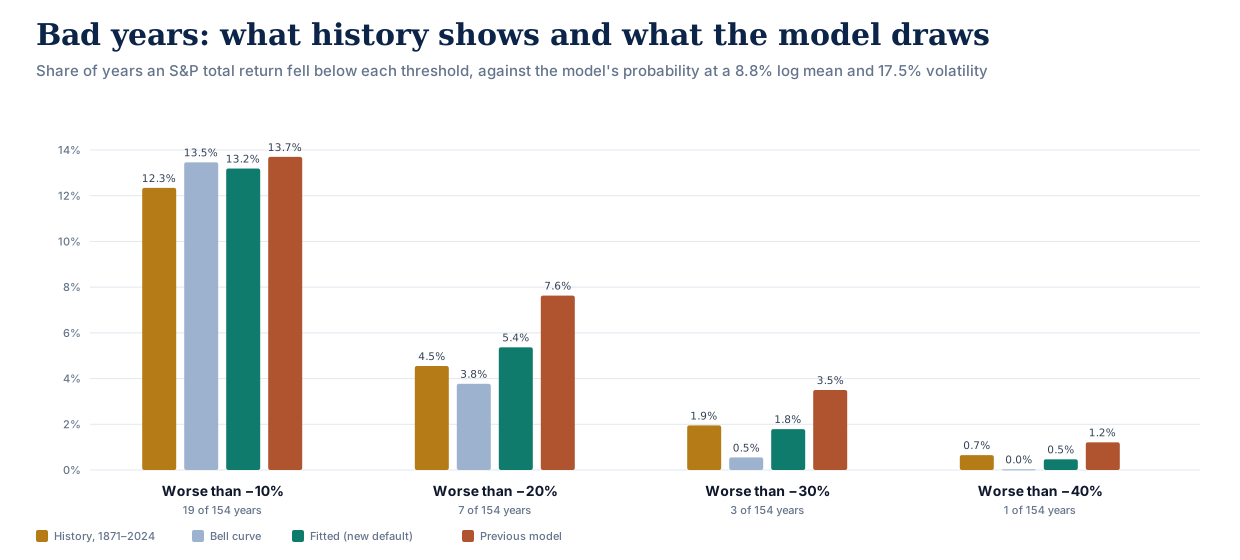
A bell curve sees a 2008-sized year about once every 180 years, far too rarely. The old shortcut saw one about every 29 years, too often. The new model sees one about every 55, against roughly one in 50 in the record: 3 such years in 154 (1931, 1937 and 2008), too few to tell those two rates apart statistically. We didn't tune the model to these rows; they are what fitting the whole distribution to 154 years of data produces.

Which assets use which shape:

• Stocks and stock-like assets (US large and small companies, international and emerging-market stocks, REITs) use the fitted shape. Only US stocks have a record long enough to fit a crash shape to; the others borrow it.
• Bonds (including long Treasuries, TIPS and international bonds) use a bell curve. Their record is mildly fat-tailed, partly because bond volatility changed several-fold between decades: about 2% a year in the 1940s, 11% in the 1980s. The best single shape we could fit matched the middle of the record but implied a bond year gaining more than 50% about once in a thousand years, and losses rarer than a bell curve allows. Nothing like that is in the record, whose best year was +33% (1982). At bonds' low volatility, the choice moves a plan's simulated success by about a tenth of a point.
• Cash, gold, commodities and managed futures use a bell curve too. Cash returns follow interest rates from year to year too closely for a one-year shape to mean much, gold's price was fixed by law for almost all of 1871–1970, and commodities and managed futures have under 60 years of data.

Strictly, "bell curve" here means each year's growth is bell-shaped on a logarithmic scale (a log-normal distribution), the standard choice in finance because it can never lose more than 100%.

Why the shape of a single year barely matters

Once the new model was in place, we asked how much a plan's result depends on the crash shape. For a 40-year-old couple spending $60,000 a year with no tax, in an 80/20 portfolio, here is the portfolio that clears a 95% simulated success target under different shapes, all with the same average return and the same volatility:

How each year's return is shaped	Portfolio needed
Plain bell curve	$1,940,000 (32.3× spending)
Fitted to history (the new default)	$1,970,000 (32.8×)
The heaviest crash tail history can't rule out	$1,970,000 (32.8×)
The old shortcut, for comparison	$2,080,000 (34.7×)

The fitted shape asks for 0.5 years of spending more than a bell curve, and the heaviest tail the record allows asks for 32.8×, essentially the same. The old shortcut, solved before both corrections and with the old default returns, needed 34.7×; most of what it added came from its extra volatility rather than its shape.

The reason is that a plan's outcome depends on many years added together, and adding years together dilutes whatever is unusual about any one of them. Picture a 20-sided die whose faces are a year's return: −30%, −15%, −10%, −5% and 0% once each; +5%, +25% and +30% on two faces each; +10%, +15% and +20% on three faces each. One roll is lopsided, much like a year of US stocks: usually a gain, sometimes a painful loss, and the worst face sits further below the average than the best face sits above it. The die averages 9.8% a year with a typical swing of 15.2%, and its lopsidedness (skewness) is −0.89, close to US stocks' −0.82. Now roll it 10 or 30 times and average the rolls:

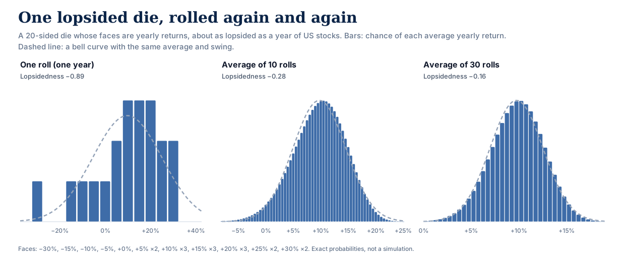
The lopsidedness fades with the square root of the number of rolls: −0.89 for one roll, −0.28 for ten, −0.16 for thirty, where a bell curve is 0. Statisticians call this the central limit theorem: add up enough independent random amounts and the total is shaped like a bell curve, whatever each amount looks like on its own. (Strictly, returns multiply rather than add. The theorem applies to their logarithms, which do add, which is why the simulator works with log returns.)

Market years work the same way. A plan's fate is decided mostly by its first 10 to 20 years, and over that many years, the lopsided shape of a single stock year is largely diluted away. Even then, how far a single year can fall still matters for how a plan feels. For whether the money lasts, three things dominate: how much the portfolio grows on average, how big the ups and downs are, and whether the bad years come early.

The same reasoning says where the shape does show through. The fewer years an outcome depends on, the less dilution there is, so short plans feel each year's shape far more than long ones. So does any question about rare events, such as a 99% success target, because a rare bad outcome is made of the few worst years rather than the typical many. The die shows this too: the far tails are the last part to even out. After 10 rolls, the average lands more than two typical swings below the middle 3.1% of the time and that far above it 1.5% of the time, against 2.3% each way on a bell curve.

Where the shape does matter

The shape is not irrelevant. It matters wherever a result depends on single years rather than on decades:

• How often big crashes happen. At the record's rate, the chance of at least one year in which US stocks lose 30% or more, somewhere in a given decade, is about 18%. The new model puts it at 17%; a bell curve at 5%. If the question is how likely a crash is during the first ten years of retirement, a bell curve understates it by a factor of about 3.
• Strict success targets. A 30-year, all-stock plan withdrawing 3% fails in 3.1% of simulated paths with the fitted shape, against 2.5% on a bell curve; at 3.5%, 5.4% against 4.8%. If you plan to a 99% standard, that is the gap that matters.
• Short, tight plans. A 10-year plan withdrawing 12% a year succeeds in 73.2% of paths with the fitted shape and 71.8% on a bell curve. Here the shape helps. With the average and volatility held fixed, a longer left tail turns some moderately bad years into rare terrible ones and makes typical years slightly better, and over a few years the typical years carry more weight.

For contrast, ordinary plans barely move: an 80/20 plan withdrawing 4% succeeds in 94.2% of paths over 30 years with the fitted shape and 94.7% on a bell curve, and in 86.7% and 86.4% over 55 years. The math section below explains why.

That changed what we built. We had planned to let you choose between milder and more severe crash shapes, and briefly did. But a setting whose label promises a harsher outcome and then barely moves the result is worse than no setting. So the shape is now a fixed part of the model, fitted to history, and the setting is about turbulence.

Market turbulence

Volatility, the size of the ups and downs, is the one market parameter history measures well. US stock volatility over 30-year stretches has ranged from about 13% to about 25% a year, and was about 17% over the whole record. The setting uses exactly that range:

Market turbulence	Ups and downs like	Stocks' typical yearly swing	A loss of 30% or worse	Portfolio needed (couple at 40, $60,000 a year)
Calmer	1871–1900, the calmest 30 years	13%	about 1 year in 200	$1,620,000 (27.0×)
As in history (default)	1871–2024, the whole record	17%	about 1 year in 55	$1,970,000 (32.8×)
Rougher	1927–1956, the roughest 30 years	25%	about 1 year in 19	$2,730,000 (45.5×)

For the same plans as in the table below: the early retiree at 4% has 92.7% simulated success with calmer markets, 86.7% as in history, and 79.2% with rougher markets; the classic retiree at 4% has 98.8%, 96.4% and 91.9%.

Turbulence changes how bumpy the ride is, not how much the portfolio grows. The average yearly growth rate (what investors call the compound return) stays at whatever the scenario says. Rougher markets still cost real money, because a run of bad years early in retirement is hard to recover from while you're withdrawing. That keeps the two dials independent: Expected returns, on the same page, sets how much the portfolio grows; Market turbulence sets how bumpy the way there is. Expected returns offers two views: History (1871–2024), the default, uses each asset's compound return over the record (US stocks 9.2% a year); Forecasters (30-yr) uses the median of the 30-year forecasts published by Vanguard, BlackRock and Verus (US stocks 5.6%, with bonds and cash a little above their history, in line with today's yields). If you expect lower returns and a rougher ride, choose both.

What it does to plans like yours

Every row below is the same household: $60,000 a year of spending, rising with inflation, no tax, rebalanced every year. The only things that vary are how long retirement lasts, how much of the portfolio is in stocks, and the starting withdrawal rate. Each cell is a 100,000-path simulation, showing the share of paths that never ran out of money under the old shortcut and the new model, with turbulence as in history. The new figures also include a second correction released at the same time: the default stock, bond and cash returns are now exactly their 1871–2024 compound rates, and default inflation is the record's 2.0%. History's stocks and bonds were bumpier than our old rounded defaults (17.5% and 6.0% volatility instead of 17% and 5%), and its stocks compounded a little less (9.2% a year instead of 9.4%). So this second correction lowers success, and takes back most of what the crash-model change adds.

Stocks 80%, bonds 20%

Withdrawal rate	30 years (retire at 65)	45 years (retire at 50)	55 years (retire at 40)
3.0%	97.8% → 98.6%	95.3% → 96.3%	94.6% → 95.3%
3.5%	96.0% → 96.9%	92.1% → 93.2%	90.7% → 91.7%
4.0%	93.4% → 94.2%	87.8% → 88.8%	86.1% → 86.7%
4.5%	89.2% → 90.5%	83.4% → 83.2%	79.6% → 80.7%

Stocks 60%, bonds 40%

Withdrawal rate	30 years (retire at 65)	45 years (retire at 50)	55 years (retire at 40)
3.0%	99.2% → 99.5%	97.3% → 98.0%	96.6% → 96.9%
3.5%	97.4% → 98.5%	94.0% → 94.9%	92.7% → 92.9%
4.0%	95.7% → 96.4%	89.5% → 90.0%	86.0% → 87.0%
4.5%	91.8% → 92.6%	83.1% → 82.9%	78.6% → 78.9%

A few patterns are worth pointing out:

• Most plans barely move. Across these 24 plans, simulated success changed by between −0.2 and +1.3 points.
• Stock-heavy plans gain a little more. The old shortcut's extra volatility was mostly in stocks, so the 80/20 plans moved +0.9 points on average against +0.6 for 60/40.
• The safest plans have the least room to change. If a plan almost never runs out of money, it can't improve much either way.

If you have a saved plan with us, find the row closest to it to get a feel for the size of the change; the exact number for your plan appears the next time you run it. Your taxes, other income and spending pattern will make your plan move by a different amount than these examples. Our walk-through of the 4% rule shows how a FIRE number is built up, step by step, on the new model.

Why we changed it

We picked the old stretch for simplicity in 2020, when the simulator was first built: a round number that clearly made bad years worse than a bell curve. We never fitted it to historical data until now. When we did, three problems showed up. It made bad years too common. It made every asset more volatile than the scenario said, because stretching the bad side widens the whole distribution. And it treated every asset the same way, although bonds' history looks nothing like stocks'.

For the mathematically curious

The model. Each year, each asset's log return is

r = μ + k·σ · (T(z) − m) / s, where T(z) = (e^{gz} − 1)/g · e^{hz²/2}

Here z is a standard normal draw, T is Tukey's g-and-h transform (Tukey 1977; Hoaglin 1985), g controls skew (negative g gives a longer left tail) and h controls tail weight. m and s are the exact mean and standard deviation of T(z), which have closed forms (Martinez & Iglewicz 1984), so μ is the expected log return (the compound growth rate) and σ the volatility, exactly. k is the turbulence multiplier: 0.749, 1, or 1.404. Assets are correlated through a Cholesky factor of their correlation matrix before the transform, so the dependence between assets is a Gaussian copula.

Why the shape washes out. For a sum of n independent years, skewness shrinks with √n and excess kurtosis with n. A plan's fate is set mostly by its first 10 to 20 years, over which stocks' single-year skewness of −0.82 shrinks to about −0.26 to −0.18. To first order (the Cornish–Fisher expansion), skewness γ moves a distribution's 5th percentile by about 0.28γ standard deviations and its 1st percentile by about 0.74γ. At a 95% success target, that is about 0.05 to 0.07 standard deviations of those years' combined return. At 99% it is roughly two and a half times as much, which is why strict targets notice the shape and ordinary ones barely do.

Choosing a distribution. We fitted the obvious candidates by maximum likelihood to annual log returns of the S&P composite, 1871–2024, and of 10-year US Treasuries, 1926–2024 (lower AIC and BIC are better).

Stocks, 1871–2024 (skewness −0.82, excess kurtosis 1.10):

Distribution	Parameters	Log-likelihood	AIC	BIC
Skew-normal (Azzalini)	3	58.5	−110.9	−101.8
Tukey g-and-h (current model)	4	58.7	−109.5	−97.3
Left-tail stretch (former model)	3	55.2	−104.5	−95.4
Student t	3	52.5	−98.9	−89.8
Normal (log-normal returns)	2	50.5	−97.1	−91.0

Bonds, 1926–2024 (skewness 0.33, excess kurtosis 1.53):

Distribution	Parameters	Log-likelihood	AIC	BIC
Tukey g-and-h (current model)	4	124.5	−241.1	−230.7
Student t	3	122.6	−239.1	−231.3
Left-tail stretch (former model)	3	119.4	−232.8	−225.0
Normal (log-normal returns)	2	118.0	−232.0	−226.8
Skew-normal (Azzalini)	3	119.0	−231.9	−224.2

The two tables point in different directions:

• Stocks' extra weight is in one tail. Their excess kurtosis comes almost entirely from big down-years, so the symmetric Student t barely beats a bell curve and the skew-normal is the most economical fit. g-and-h fits as well, but its maximum-likelihood tail weight is h = 0.00, so it pays a penalty for a parameter it doesn't use. This matches a well-known stylized fact: daily returns have very heavy tails that largely wash out by the time they add up to a year, while the asymmetry survives (Cont 2001).
• Bonds are fat-tailed on both sides, and only mildly skewed. A skew-normal can only add skew, and its excess kurtosis can never exceed about 0.87, so for bonds it gains almost nothing over a bell curve. Student t, built for symmetric fat tails, does well and is best by BIC, which penalises the extra parameter more; g-and-h is best by AIC, but only at the edge of the model, and its tails fail the check below. Bonds use the log-normal.

For stocks, then, the skew-normal and g-and-h fit equally well. We use g-and-h for a practical reason: it is a closed-form, monotone transform of a standard normal draw. The simulator already produces each asset's correlated normal draw, and g-and-h converts it directly. Because the transform is monotone, the rank correlation between any two assets carries through exactly (the ordinary, linear correlation shifts slightly), and the simulator's fast and slow paths stay in exact agreement. A skew-normal has no such transform: you need either its inverse distribution function (no closed form) for every asset and year, or a two-draw construction that changes how assets move together. g-and-h also has a track record in risk measurement: bank-regulatory research on operational-risk capital found it fit loss data as well as distributions designed for heavy tails (Dutta & Perry, Federal Reserve Bank of Boston, 2006).

How each asset was fitted.

• Stocks: maximum likelihood on 1871–2024, g = −0.27, h = 0.00. Against a plain log-normal, the likelihood-ratio statistic is 16.4 (the 5% critical value is 3.84). International, emerging-market and small-company stocks and REITs borrow this shape; their own records are either too short to say anything about crashes, or, for small companies' 99 years, not distinguishable from a bell curve.
• Every fit must reproduce the record's own skewness and kurtosis. A likelihood only sees the years that happened, so a shape can match them well and still imply tails nothing in the record resembles. We accept a fitted shape only if its exact skewness and excess kurtosis (closed forms from Martinez & Iglewicz) fall inside the 95% bootstrap intervals of the record's. Stocks pass: the fit implies skewness −0.84 and excess kurtosis 1.28, against intervals of [−1.25, −0.31] and [−0.40, 2.52].
• Bonds fail it. Maximum likelihood on 1926–2024 runs to the edge of the model, and Hoaglin's quantile ("letter value") estimator, which is robust to that, gives g = 0.42, h = 0.16. That shape implies skewness 4.63 and excess kurtosis 164, against intervals of [−0.44, 1.11] and [0.07, 2.96]. Part of the record's fat tails comes from bond volatility changing between decades, which no single shape represents; within each decade, bond skewness is indistinguishable from zero. (Before 1926 our bond series is reconstructed from 10-year yields, a quarter as volatile as measured returns afterwards, so we don't fit it at all.) Long Treasuries, TIPS and international bonds follow bonds.
• Everything else (cash, gold, commodities, managed futures) uses the plain log-normal, for the reasons above.
• h is capped below ¼. Above that, the g-and-h distribution has infinite kurtosis, which a simulator should not draw from.

Turbulence. The multipliers are ratios of US stock volatility in the calmest and roughest 30-year windows of 1871–2024 to the volatility of the whole record: 13.1% ÷ 17.5% and 24.6% ÷ 17.5%, rounded to 0.75 and 1.40. One multiplier scales every asset, which is a simplification: history's roughest era for stocks was a calm one for bonds (2.8% a year in 1927–1956), and bonds' roughest 30 years came later (1980–2009, 9.9% a year). So Rougher is a stress test for the whole portfolio, not a replay of one era. With the simulator's default 6% bond volatility, it takes bonds to about 8.4%, between their measured average since 1926 (7.4%) and their roughest 30 years (9.9%). Volatility is the parameter a long record estimates best; expected returns are much harder (Merton 1980), which is why the expected-return presets matter even more than this one.

What this model does not do.

• The fitted stock tail reaches past the record. A g-and-h shape keeps stretching beyond the worst year observed. In the model, the worst stock year in a thousand is a loss of about −50%, against −36% on a bell curve; the worst year on record is −44% (1931). Years like that are too rare to move a plan's success rate, but they are extrapolation, not evidence.
• Annual data hides intra-year drawdowns. 1987's crash, for instance, ended the year with a gain. For a retiree withdrawing once a year, annual returns are the relevant unit, but the tail of daily returns is much heavier.
• It is US data, with the survivorship bias that implies. The US was one of the best-performing markets of the last 150 years. Across 17 countries, Wade Pfau found that a 4% withdrawal would have been safe in only 4; across 38 developed markets, Anarkulova, Cederburg, O'Doherty and Sias estimate 2.31% for a couple accepting a 5% chance of ruin.
• Assets crash together only as often as their correlation implies. A Gaussian copula has no extra "everything falls at once" behaviour, while real correlations tend to rise in bad markets (Longin & Solnik 2001). A t-copula is a natural next step.
• Years are drawn independently. There is no momentum or mean reversion, so bad years don't cluster the way 1929–1932 did, and recoveries are not built in either. Rougher raises the size of every year's swings; it does not create multi-year bear markets. On US data the net effect of independent draws is caution, not optimism: they produce long losing stretches more often than the record did, which is the largest single step in our walk-through of the 4% rule.
• 154 years is still a small sample for events that happen once every few decades.

The analysis is reproducible. The scripts are published as tail_calibration.py and tail_family_comparison.py, the series they read as CSV (stocks, bonds, small-company stocks, long Treasuries; each file's header gives its sources), and their full output as JSON (calibration, comparison). If you get a different answer from the same data, we want to hear about it.

References. Tukey, J. W. (1977), Modern techniques in data analysis. Hoaglin, D. C. (1985), "Summarizing shape numerically: the g-and-h distributions", in Exploring Data Tables, Trends, and Shapes, Wiley. Martinez, J. and Iglewicz, B. (1984), "Some properties of the Tukey g and h family of distributions", Communications in Statistics: Theory and Methods 13(3). Azzalini, A. (1985), "A class of distributions which includes the normal ones", Scandinavian Journal of Statistics 12(2). Merton, R. C. (1980), "On estimating the expected return on the market", Journal of Financial Economics 8(4). Dutta, K. and Perry, J. (2006), "A tale of tails", Federal Reserve Bank of Boston Working Paper 06-13. Cont, R. (2001), "Empirical properties of asset returns: stylized facts and statistical issues", Quantitative Finance 1(2). Longin, F. and Solnik, B. (2001), "Extreme correlation of international equity markets", Journal of Finance 56(2).

What happens next

• Your saved plans: the next run of each saved scenario uses the new model with turbulence as in history. Past runs, reports and shared links are unchanged.
• If a saved plan moved by 3 points or more, or crossed 80%, 90% or 95% simulated success in either direction, we'll email you that plan's before-and-after numbers, once. Better news matters as much as worse: it can mean you're closer to your goal than you thought. You can turn these correction notices off in your account settings or from the email itself.
• Your own view of markets: if you expect the next decades to be rougher, or calmer, than the last 154 years, set Market turbulence on your scenario's Portfolio page. If you also expect lower long-run returns, set Expected returns there to Forecasters (30-yr).

The methodology page has the full description of the simulator, including what it doesn't model.