
The 4% rule says you can withdraw 4% of your starting portfolio, raise it with inflation every year, and not run out. Flip it over and you get the FIRE community's favourite number: save 25× your annual spending.
Most arguments about that number are arguments about different questions. William Bengen's 1994 study, Determining Withdrawal Rates Using Historical Data, asked a precise one: for a 30-year retirement in a 50/50 portfolio of US stocks and intermediate Treasuries, what is the highest inflation-adjusted withdrawal that never ran out of money in the historical record, before tax? Someone retiring at 40, holding mostly stocks, comfortable with some risk, paying tax somewhere, is asking a different question, and gets a different answer.
So we rebuilt the answer one assumption at a time. We started by reproducing Bengen's result, then changed exactly one thing per step and asked Retirement Lab for the smallest portfolio that still met that step's standard. Every number below is a production simulation, and every row links to the run that produced it, so you can open it, check the inputs, and change them.
Here is where it ended up, for a household spending $60,000 a year:
- Bengen's question, reproduced: 25.2× spending, a 3.97% withdrawal rate. For the question it asked, the 4% rule holds up.
- Retiring at 40 instead of 65, replaying history: between 24.0× and 29.3×, depending on the portfolio and how much failure you accept.
- Treating each future year as an independent draw from history: 32.3×. This is the biggest single step, and the one most worth arguing about.
- Giving returns history's crash shape: 32.8× with no tax, barely more than a bell curve. Turbulence matters more: markets as rough as 1927–1956 push it to 45.5×. With tax, it ranges from about the same (a US taxable account) to 49.8× (the Netherlands), depending on where you live and how you hold the money.
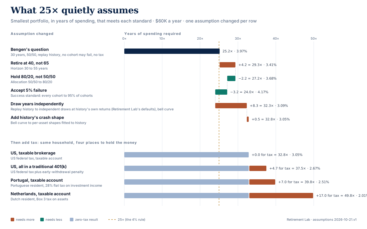
| Step | What changed | Success standard | Required portfolio | Years of spending | Withdrawal rate |
|---|---|---|---|---|---|
| 1 | Bengen's question | every historical cohort | $1,510,000 | 25.2× | 3.97% |
| 2 | Retire at 40: 55 years, not 30 | every historical cohort | $1,760,000 | 29.3× | 3.41% |
| 3 | Hold 80/20, not 50/50 | every historical cohort | $1,630,000 | 27.2× | 3.68% |
| 4 | Accept 5% failure | 95% of historical cohorts | $1,440,000 | 24.0× | 4.17% |
| 5 | Draw each year independently from history | 95% of simulated paths | $1,940,000 | 32.3× | 3.09% |
| 6 | Give returns history's crash shape | 95% of simulated paths | $1,970,000 | 32.8× | 3.05% |
Steps 1 to 6 pay no tax: the household is resident in, and a citizen of, the UAE, which levies no personal income tax. Tax comes last, so that every step before it isolates one assumption about markets and risk.
Step 1: reproducing Bengen
Retirement Lab's historical mode replays actual annual US returns and inflation: S&P composite total returns, intermediate Treasuries, and CPI-U, from 1871 through 2024. Each start year is one retiree, or cohort. A 30-year retirement gives 125 cohorts, from 1871 to 1995.
With Bengen's settings — 30 years, 50/50, rebalanced every year, no tax, no cohort allowed to run out — the smallest portfolio that funded every cohort was $1,510,000: 25.2× spending, a 3.97% withdrawal rate. Bengen's answer, on the 1926–1992 data available to him, was about 4%. This run adds the 19th century and three more decades, and the answer barely moves.
That is worth saying plainly, because the 4% rule gets dismissed a lot: for the question it asked, it holds up. The problems start when it is used to answer other questions.
The 4% rule is the worst year, not a typical one
The single number hides a distribution. For every start year, we searched for the highest withdrawal rate that never ran out of money:
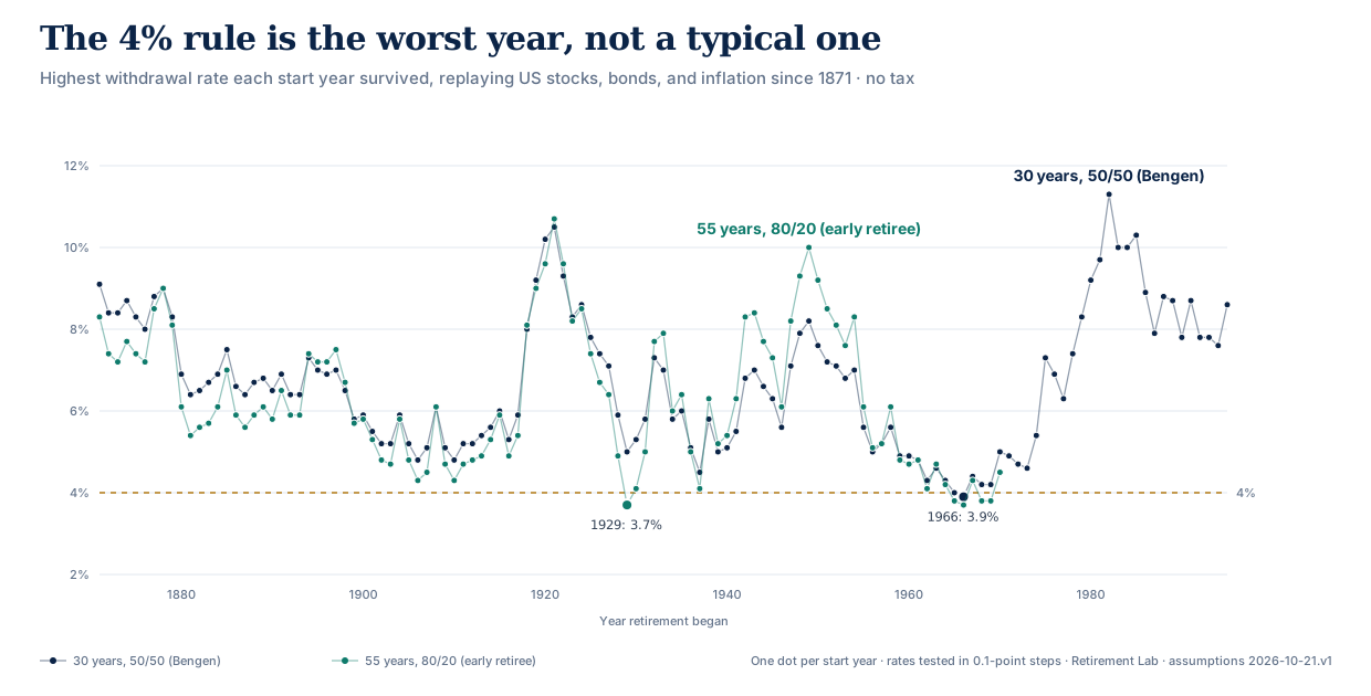
For Bengen's 30-year retiree, the median start year could have withdrawn 6.6% and the best could have withdrawn 11.3%. The 4% rule is the floor, set by a handful of retirees who started in the mid-1960s and met a decade of high inflation and flat real returns: 1966 (3.9%), 1965 (4.0%), 1968 (4.2%), and 1969 (4.2%).
Two things follow. First, in a typical market 4% leaves a lot unspent: half of all start years could have withdrawn 6.6% or more for 30 years. Second, the rule's safety comes entirely from planning for the worst case on record. Everything that follows is about whether the worst case on record is a good enough guide.
Steps 2–4: what history says about retiring at 40
Lengthen the horizon to 55 years (retiring at 40, planning to 95): 29.3×, a 3.41% withdrawal rate. A longer retirement leaves less room to spend principal, and gives a bad sequence more time to compound. This step is the one most early retirees already know about. It is consistent with what Karsten Jeske found for long horizons in his Safe Withdrawal Rate series, from a different dataset and method.
Hold 80/20 instead of 50/50: 27.2×. Over 55 years, the extra equity return outweighs the extra volatility in the historical record. That is why most FIRE portfolios are equity-heavy, and it is the first step in this article that lowers the number.
Accept 5% failure instead of none: 24.0×, a 4.17% withdrawal rate — under 25×. With 100 cohorts, a 95% standard means five may fail. At this portfolio those five were 1929, 1965, 1966, 1968, and 1969: the 1929 crash, and the same inflationary mid-to-late-1960s starts that set Bengen's floor.
This is the most surprising result in the study. On the historical record alone, an early retiree with an 80/20 portfolio who accepts a 5% failure rate needed less than 25×. If the next 55 years replay one of the last 150 years' actual sequences, the 4% rule is not obviously too aggressive for an early retiree.
Whether that is a safe assumption is the next step.
Steps 5 and 6: from history to a model
A historical backtest has a problem that gets worse with the horizon: there is not much history. Since 1871 there are fewer than three non-overlapping 55-year periods, and the cohorts above share most of their years. A Monte Carlo model trades that problem for another one — you have to choose its assumptions — but it lets you see sequences the record happens not to contain.
Step 5: draw each year independently from history. We switched to a simulation that draws every year's stock and bond returns independently, from a distribution with history's own figures, all from the same 1871–2024 series: stocks compounding at 9.2% a year with 17.5% volatility, bonds at 4.4% with 6.0%, and 2.0% inflation. These are also Retirement Lab's defaults, which are computed from that series. To start, the distribution is a plain bell curve (log-normal). Result: 32.3×, up from 24.0×. This is the largest step in the waterfall.
Same average returns, same volatility, very different answer. The reason is sequencing. History's actual 55-year runs were kinder than random draws with the same averages: in the record, a terrible decade has tended to be followed by a recovery, while independent draws allow bad decades to pile up back to back. Whether that pattern is a feature of markets (economists call it mean reversion and have argued about it for decades) or a lucky small sample is genuinely open. If you believe in it, the replay steps are your guide; if you don't, the model steps are. We think a plan for a 55-year retirement should not rely on the friendlier answer.
History's averages are not a forecast, though, and the expected return is the assumption people disagree about most. Published 10-year forecasts are well below history: Vanguard's model run of June 30, 2026 puts US stocks at 4.2%–6.2% a year, and J.P. Morgan's 2026 long-term assumptions at 6.7% over 10–15 years. The few forecasters who look 30 years ahead are barely more optimistic: Vanguard's 30-year median for US stocks is 5.6%, Verus's 5.6%, and BlackRock's 8.4%. Retirement Lab's Forecasters (30-yr) return preset uses the median of those three for every asset class. And even a 10-year forecast covers the first decade of retirement, which is exactly where a bad sequence does its damage. So here is the step-6 model with every other assumption fixed and only the stock return changed:
| Stocks compound at (nominal) | Required portfolio | Years of spending | Withdrawal rate |
|---|---|---|---|
| 5.0% | $4,030,000 | 67.2× | 1.49% |
| 6.0% | $3,320,000 | 55.3× | 1.81% |
| 7.0% | $2,770,000 | 46.2× | 2.17% |
| 8.0% | $2,360,000 | 39.3× | 2.54% |
| 9.2% (1871–2024) | $1,960,000 | 32.7× | 3.06% |
| 10.0% | $1,760,000 | 29.3× | 3.41% |
Bonds stay at a compound 4.4% and inflation at 2.0%; each row uses the step-6 crash assumption.
If you take one table from this article, take this one. Over a 55-year retirement, each point of expected stock return is worth between four and twelve years of spending (more at the low end), and the published 10-year forecasts above sit at the expensive end of this table. A FIRE number is mostly a bet on future returns, and it is better to make that bet explicitly than to inherit it from a rule of thumb.
Step 6: give returns history's crash shape. Annual stock returns are not bell-shaped: crashes are larger and more common than a bell curve allows, and big up-years are rarer. The simulator now shapes stock returns with a Tukey g-and-h distribution fitted to that history (bonds stay on a bell curve), which keeps the average return and volatility exactly as configured and only changes how often extreme years happen. For US stocks, the result draws years worse than −20%, −30% and −40% at about the rates history did:
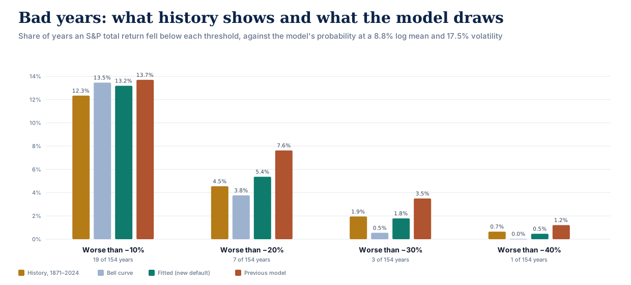
Result: 32.8×, a 3.05% withdrawal rate. This is the article's zero-tax answer for a 40-year-old.
Notice how little that moved: 32.3× to 32.8×. With the heaviest crash tail the 154-year record can't statistically rule out, the household needs 32.8×, essentially the same. Over 55 years, the shape of any single year mostly averages out; what survives is the average return, the size of the swings and their order.
The size of the swings does matter. With ups and downs as large as in 1927–1956, the roughest 30 years for US stocks on record, the same household needs 45.5×; as small as in 1871–1900, the calmest, 27.0×. Both keep the compound return fixed, so the whole difference is volatility and sequence risk. Retirement Lab offers these as Market turbulence on each scenario's Portfolio page.
That is also why the model Retirement Lab used until October 2026 needed 34.7× here. It stretched bad years by a fixed factor of 2.0, which, at the same stock parameters, draws a 30%-plus loss about 1.8 times as often as history did, and, more importantly, quietly made stocks about 18% more volatile than configured. We replaced it after this analysis; how we model market crashes explains the choice, the fit, and what it did to existing plans.
What if spending can flex?
Every row so far spends exactly the same real amount every year, whatever markets do. Real retirees don't: they skip the big trip in a bad year. A small amount of flexibility goes a long way. With one simple rule — spend $60,000, but drop to $45,000 (inflation-adjusted) in any year the portfolio is below half its starting value — the step-6 household needed 31.2× instead of 32.8×.
The 4% rule's rigidity is one of its most criticized assumptions, and it cuts against early retirees most, because a long retirement gives the most room for adjusting.
Then add tax
Everything above was pre-tax. Here is the same step-6 household, holding the same money four different ways:
| Where and how the money is held | Required portfolio | Years of spending | Withdrawal rate | Median first-year tax |
|---|---|---|---|---|
| No tax (UAE) | $1,970,000 | 32.8× | 3.05% | none |
| US, taxable brokerage account | $1,970,000 | 32.8× | 3.05% | none |
| US, all in a traditional 401(k) | $2,250,000 | 37.5× | 2.67% | $11,300 |
| Portugal, taxable account | $2,390,000 | 39.8× | 2.51% | €13,700 |
| Netherlands, taxable account | $2,990,000 | 49.8× | 2.01% | €54,900 |
A US taxable account costs almost nothing at this spending level. A married couple living on $60,000 of dividends and long-term gains stays inside the standard deduction and the 0% capital-gains bracket, so it paid no federal tax in year one. (Any gap to the no-tax row within a $10,000 search step is sampling noise.)
The same money in a traditional 401(k) costs about 5 years of spending. Every withdrawal is ordinary income, and before 59½ it also carries the 10% early-withdrawal penalty. This row assumes no planning around that; our account-mix study covers Roth conversion ladders and how much they recover.
Portugal's 28% flat tax on investment income adds about 7 years (special regimes for new residents are not applied). The Netherlands adds about 17, because Box 3 taxes a deemed return on assets rather than actual income, so the charge does not fall when you spend less; in year one it was €54,900. The Dutch rules are due to change in 2028, and the simulation applies the 2026 rules throughout.
What this does not say
This is a decomposition of one household's number, not a recommendation and not a forecast of your outcome.
- US history only. The historical steps replay US markets, which were among the best-performing in the world over this period. Across 17 countries, Wade Pfau found that 4% would have been safe in only 4. Across 38 developed markets, Anarkulova, Cederburg, O'Doherty and Sias estimate 2.31% for a couple accepting a 5% chance of ruin.
- No other income. No Social Security, pensions, part-time work or home equity. For a 40-year-old couple, Social Security alone could cover a meaningful share of later spending.
- The model is simple on purpose. Returns are drawn independently each year, with no momentum or mean reversion. Stock and bond volatility are fixed at 17% and 5% (history: about 17.5% and 6%) except in the two turbulence rows, the two are uncorrelated (history: 0.04), and inflation is a constant in the Monte Carlo steps. The historical steps carry real inflation shocks; the model steps do not.
- No fees. None of the cases deducts fund or advisory fees. A 0.5% annual fee is roughly a half-point lower return in the sensitivity table.
- Order matters. The size of each step depends on what came before it. The endpoints are robust; the attribution between neighbouring steps is a choice.
- Resolution. Portfolios are searched in $10,000 steps, about 0.17 years of spending. Monte Carlo steps use 100,000 paths; repeat runs land within about one grid step of each other, so differences of 0.2 years between neighbouring rows are noise.
How it was run
Every figure is the smallest portfolio, on a $10,000 grid, whose own production run met that step's standard, and each link opens that exact run. Historical steps are deterministic: success is the share of start years that never ran out, so the search is an exact bisection. Monte Carlo steps use 100,000 simulated paths per run and publish the first grid point whose own run reached 95%.
The simulator draws log returns, so its expected returns are mean log returns: history enters the model as the mean of log returns (equivalently, the compound rate), not the arithmetic average, which would overstate it by about two points a year. Retirement Lab's defaults are those figures rounded to 0.1 point, computed from the same series. The crash shape in step 6 is a Tukey g-and-h distribution fitted by maximum likelihood to the simulator's own 1871–2024 stock series; bonds use a log-normal, because no single shape we could fit was consistent with their record; the method, the alternatives we compared, and its limits are in how we model market crashes. The "previous model" figure was solved on assumptions 2026-10-14.v1, before that change, and is shown for comparison only.
The household is a married couple spending $60,000 a year in today's money, adjusted for inflation every year, rebalanced annually, and planning to age 95. Steps 1–7 are resident and citizens in the UAE so that no tax applies; the tax cases are US, Portuguese and Dutch residents who are citizens of the same country. Historical data comes from Retirement Lab's 1871–2024 annual series: S&P composite total returns (Shiller, then Damodaran from 1926), intermediate Treasuries (a GS10 duration approximation, then Ibbotson from 1926), and US CPI-U. All runs used Retirement Lab assumptions version 2026-10-21.v1.
The cohort chart runs each historical household at withdrawal rates from 2.5% to 12% in 0.1-point steps, and records, for each start year, the highest rate it survived.
The full dataset — every step's payload, success standard, production run, share link, the per-cohort results, and the historical figures used in step 5 — is available as CSV and JSON under CC BY 4.0. Please check the numbers.
Run it with your own inputs
The useful version of this exercise is your own: your spending, your horizon, your accounts, your tax residence, and your view of future returns. Open any step above and fork it, or start a new Retirement Lab scenario from your own numbers. The methodology page documents the return model, historical mode, and each country's tax rules and known simplifications.